Forecast cloud costs

Forecasting uses your historical data to predict what your future cloud spend will be. Accurate forecasting of cloud resource usage helps you align resource allocation to other FinOps capabilities and drives good business decisions.

DoiT forecasting

DoiT offers enhanced forecasting that is reliable and configurable. Our machine learning model incorporates diverse forecasting models to accommodate various types of time series data and allows forecasting at different granularity levels.

There are several advantages to forecasting cloud costs:

Cost optimization: By predicting future cloud usage, you can identify areas to optimize your cost. This could mean turning off unused resources, right-sizing instances, and other enhancements.
Improved budgeting: Accurate forecasting helps you create realistic budgets for cloud expenses and allocate resources effectively, avoiding unexpected cost overruns.
Better decision-making: Forecasting provides valuable data for you to make better decisions about cloud usage. For example, you can determine whether its more cost-effective to scale up your cloud resources or invest in on-premises infrastructure.
FinOps best practices: Cloud cost forecasting is a core principle of FinOps. By forecasting cloud costs, you make sure you're getting the most value out of your cloud investments.

Accuracy

We continuously refine our forecasting system's data processing and modeling capabilities to improve accuracy across all time intervals. Forecasting accuracy is mainly influenced by two factors:

Seasonality: At relevant time intervals, particularly hourly and daily, you can observe recurring cost fluctuations at different times of the day or week. When we detect such a pattern, we incorporate it into the forecast to improve accuracy.
Outlier handling: Time series can generally be decomposed into trend, seasonality — where relevant — and residuals. Outliers in the residual errors can influence forecasting in a way that's not representative of the series as a whole. We mitigate the effect of such outliers and better capture essential patterns in the data.

The Historical data time range is the model's training window, affecting the model's accuracy. Set the time range, taking the following into consideration:

Match the window to current behavior: A longer history is preferrable if it reflects current behavior. However, if your spend pattern changed significantly at some point (like, a migration, new workloads, cost optimization), a shorter, stable time span with the current behavior is better.
Include at least one full cycle of your dominant pattern: If you have weekly patterns (weekday/weekend differences), include at least 2–3 full weeks. If you have monthly seasonality, include at least 2–3 full months. The shorter the historical period, the more speculative the forecast becomes.

Forecasts include confidence intervals (upper and lower bounds) that widen the further out you project. Rely on monthly forecasts rather than quarterly, because the granularity of the training data is daily and thus much more nuanced.

Historical data

By default, forecast settings auto-fill time intervals based on the report Time Range and Time Interval.

Select Historical data time range or Forecast horizon to set the time range using presets, such as Last 7 days or Next 14 days, or custom Fixed Dates with explicit start and end dates.

Time periods

The system requires at least two data points at your selected time interval, but that only yields a rough projection. For more reliable results, use the minimum recomendations listed below.

There is a maximum number of supported periods per time interval. For custom date ranges, the combined span of all selected periods must stay within the limits below.

Time period	Maximum historical periods for the forecast	Maximum forecast periods	Minimum recommended historical periods
Hourly	1000	1000	168
Daily	500	100	30
Weekly	100	52	4
Monthly	36	12	3
Quarterly	12	4	4
Annual	6	3	3

Granularity

DoiT forecasting supports two levels of granularity:

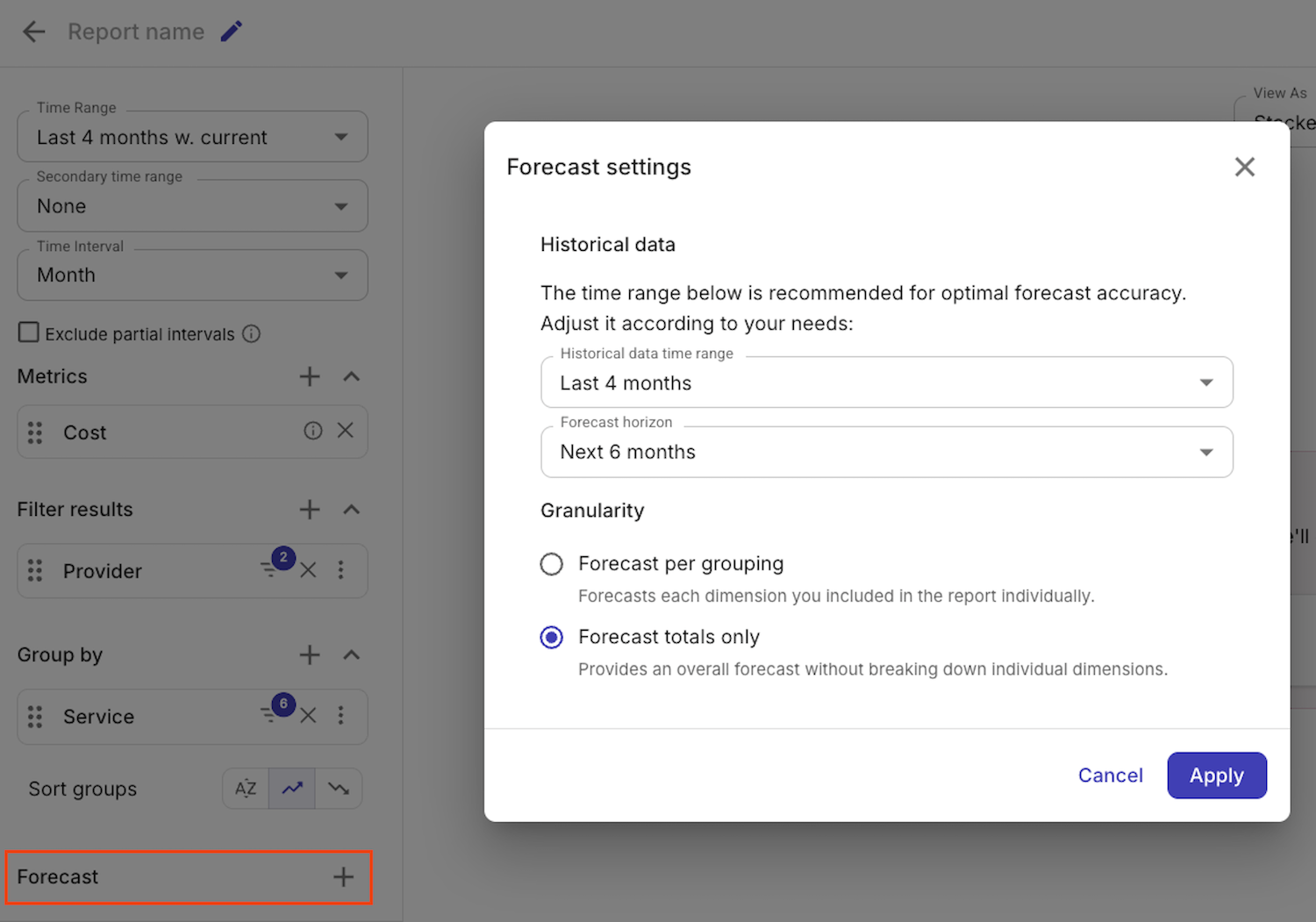
Forecast totals only: Provides an overall forecast without breaking down individual dimensions.
Forecast per grouping: Provides forecasts for each dimension included in the report's Group by configuration.

If your report is grouped by a large number of dimensions–say, more than a dozen–then the Forecast totals only option is recommended.

Choosing Forecast per grouping in such cases may result in an overcrowded report. This can be especially concerning for the last period in a report's specified Time Range. When the last period contains both historical data and forecasts, each dimension (grouping) will show two parts: the actual value so far (historical) and the forecast.

When using Forecast per grouping, each group needs enough points in range; sparse groups get noisy forecasts and confidence bounds. With limited history, Forecast totals only (or fewer, coarser groups) is usually more reliable.

See the example below for the differences caused by the levels of granularity.

Example: Forecasting service costs

This example demonstrates how to:

Create a Cloud Analytics report to forecast the spend of multiple services for a custom date range.
Change the forecast settings to see both the overall forecast and the breakdown by services.

To forecast service costs:

Create a new report in the DoiT console.
For the Time Range, select the last 4 months with the current month; for the Time Interval, select Month.

In reality, you can change these settings according to your business objectives, though you need to keep in mind the Forecasting time periods restrictions.
For the Group by option, select Service, and then filter services to include only those in which we're interested.
Select the plus icon next to Forecast to add a new forecast. The Forecast settings dialog opens, where the suggested time intervals are auto-filled based on the Time Range and Time Interval of the report.
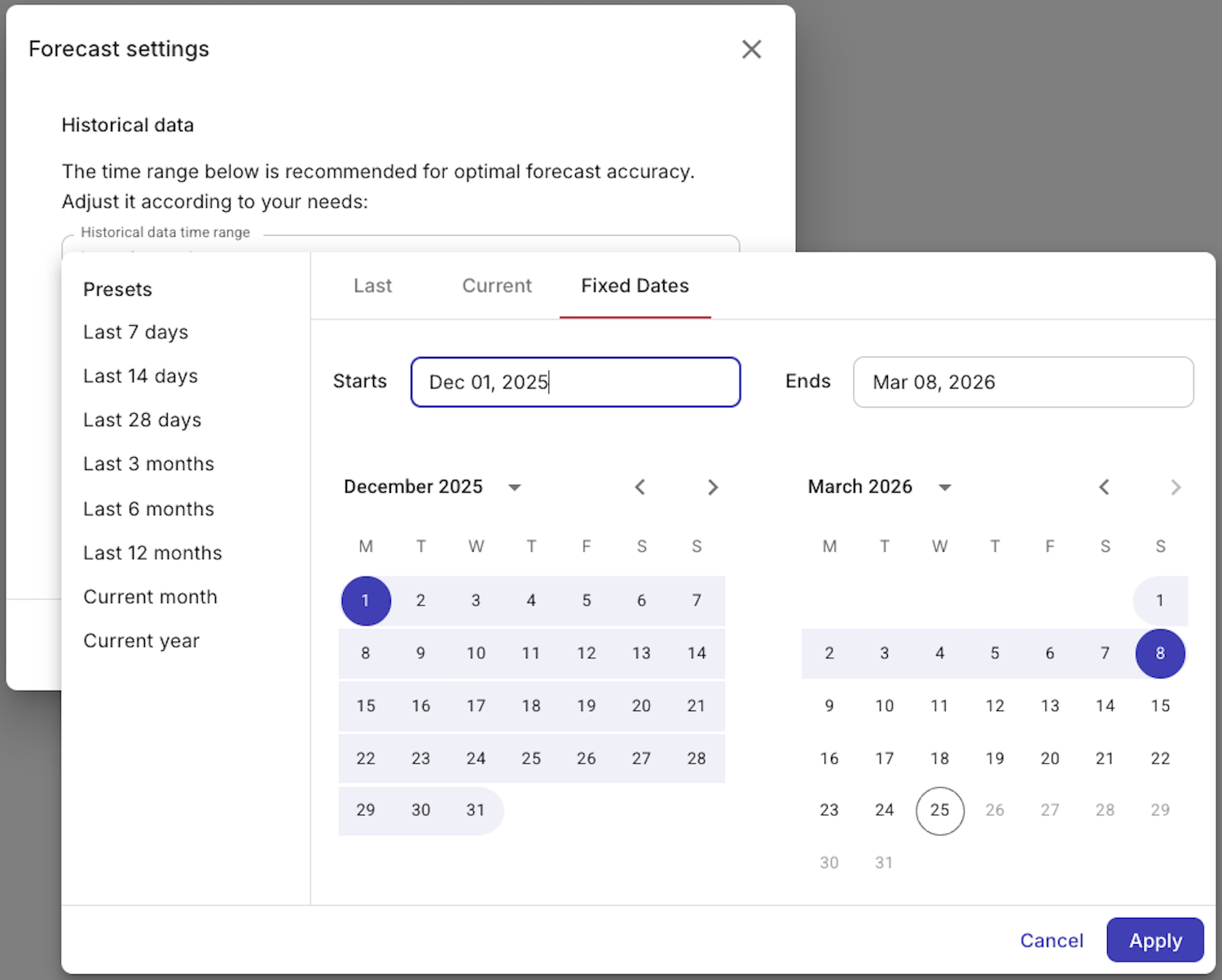
Select Historical data time range > Fixed Dates and set it to one month and one week (in this example, Dec 01, 2025 to Mar 08, 2026). Select the Forecast horizon and set it to 4 months.

These intervals can be set according to your business objectives, though keep in mind the Forecasting time periods restrictions.
Select Apply to save the settings, and then run the report.

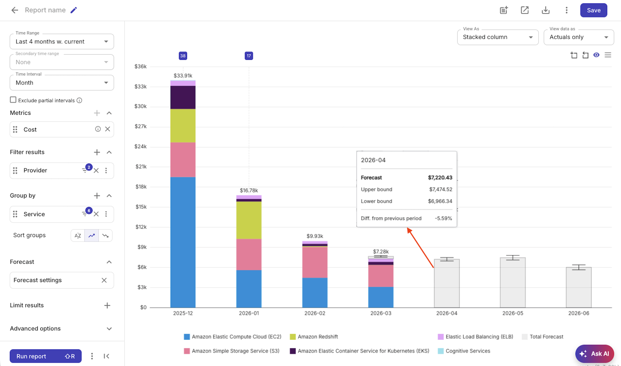
The screenshot below shows the result using the Forecast totals only granularity. Moving your mouse over a column reveals the relevant numbers.
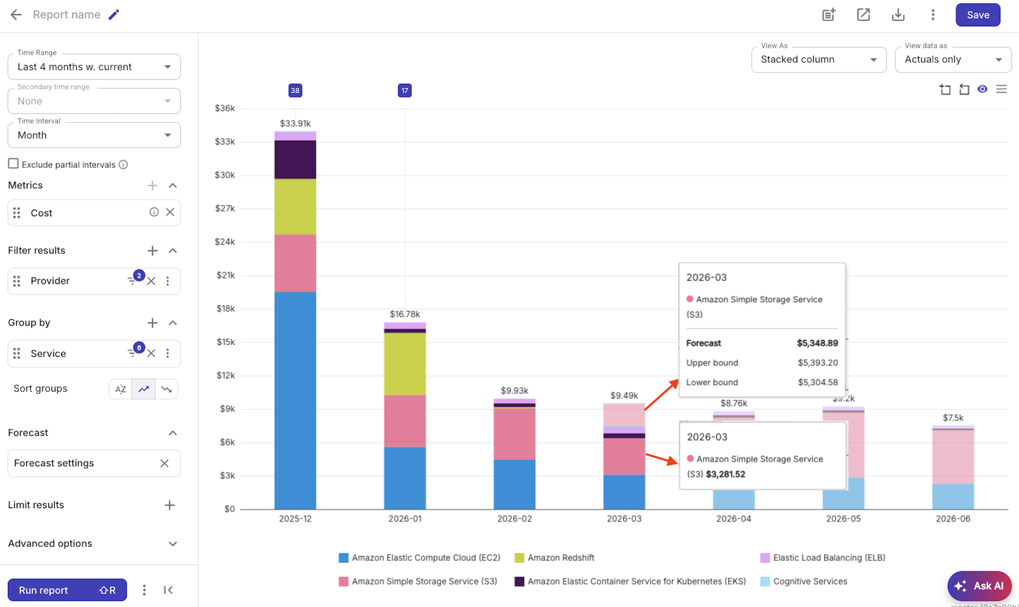
To break down the forecast per service, select Forecast settings, change the granularity to Forecast per grouping, apply the change, and then run the report again.

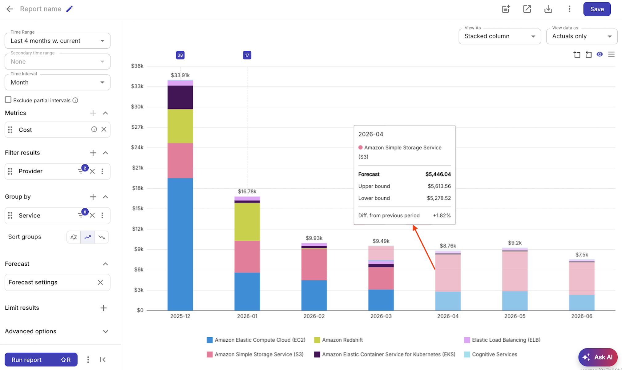
Note that in the 2026-03 column (the last period in the report's Time Range), each service has two segments, the actual and the forecast.